The origin and application of graph autoencoder

"Variational Graph Auto-Encoders" published by Kipf and Welling in 16 years proposed a graph-based (variational) auto-encoder Variational Graph Auto-Encoder (VGAE). Since then, the graph auto-encoder has relied on its simple encoder-decoder The structure and efficient encode capability have come in handy in many fields.

This article will first analyze in detail the paper "Variational Graph Auto-Encoders" that first proposed graph auto-encoders, and analyze it from the following perspectives:

The idea of VGAE

The encoder and decoder stages of GAE without variational stages

VGAE with variational stages

How to go from determining the distribution to sampling from the distribution

Experimental effect analysis

Then I will introduce two more articles on how to apply the graph autoencoder.

Variational Graph Auto-Encoders

Paper Title: Variational Graph Auto-Encoders

Paper source: NIPS 2016

Link to the paper: https://arxiv.org/abs/1611.07308

1.1 Overview of the paper

First, briefly describe the intention and purpose of the graph autoencoder: It is not easy to obtain appropriate embeddings to represent the nodes in the graph, and if you can find the appropriate embedding, you can use them in other tasks. VGAE can obtain the embedding of the nodes in the graph through the encoder-decoder structure to support the next tasks, such as link prediction.

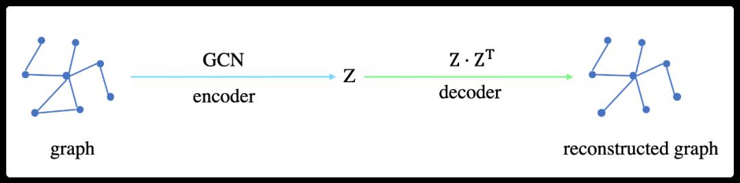
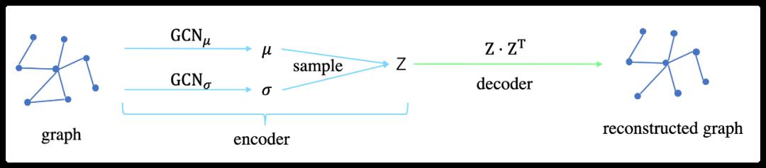
The idea of VGAE is very similar to the variational autoencoder (VAE): using latent variables, let the model learn some distributions (distribution), and then sample the latent representations (or embedding) from these distributions. This process It is the encode stage.

Then use the obtained latent representations to reconstruct the original image. This process is the decode stage. However, the encoder of VGAE uses GCN, and the decoder is a simple form of inner product.

The following specifically explains the Variational Graph Self-Encoder (VGAE). Let me talk about GAE, which is a graph autoencoder (without variation).

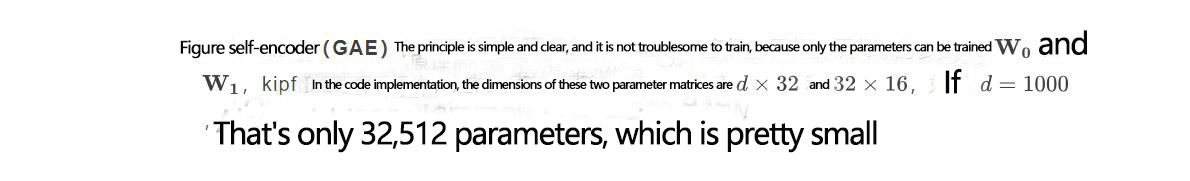
1.2 Picture self-encoder (GAE)

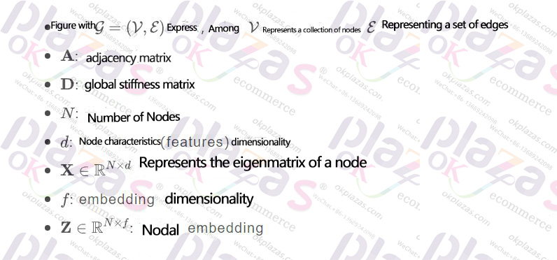
The unified specification stipulates several notations as follows:

1.2.1 Encoder

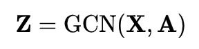
GAE uses GCN as an encoder to get the latent representations (or embedding) of nodes. This process can be expressed in a short line of formula:

How to define the function GCN? kipf is defined in the paper as follows:

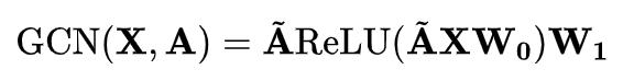
In short, here GCN is equivalent to a function that takes node features and adjacency matrix as input and node embedding as output. The purpose is only to get embedding.

1.2.2 Decoder

GAE uses inner-product as a decoder to reconstruct the original image:

1.2.3 How to learn

A good Z should make the reconstructed adjacency matrix as similar as possible to the original adjacency matrix, because the adjacency matrix determines the structure of the graph.

Therefore, GAE uses cross entropy as the loss function during training:

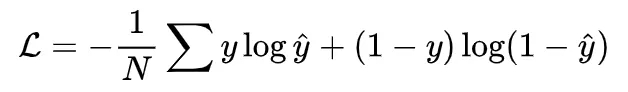
It can be seen from the loss function that the adjacency matrix (or the reconstructed graph) that is expected to be reconstructed is closer and more similar to the original adjacency matrix (or the original graph), the better.

1.2.4 Summary

The following is VGAE (Variational Graph Self Encoder).

1.3 Variational graph autoencoder (VGAE)

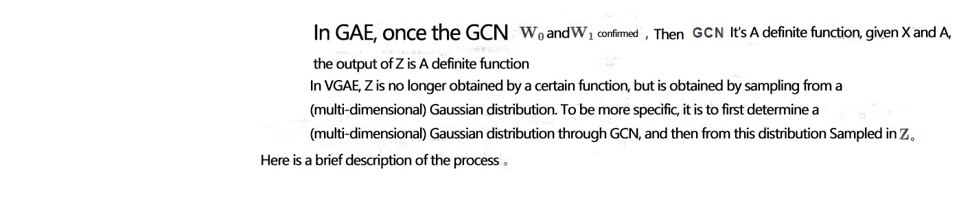
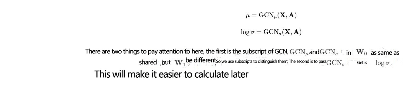
1.3.1 Determine the mean and variance

The Gaussian distribution can be uniquely determined by the second moment. Therefore, to determine a Gaussian distribution, you only need to know the mean and variance. VGAE uses GCN to calculate the mean and variance respectively:

1.3.2 Sampling

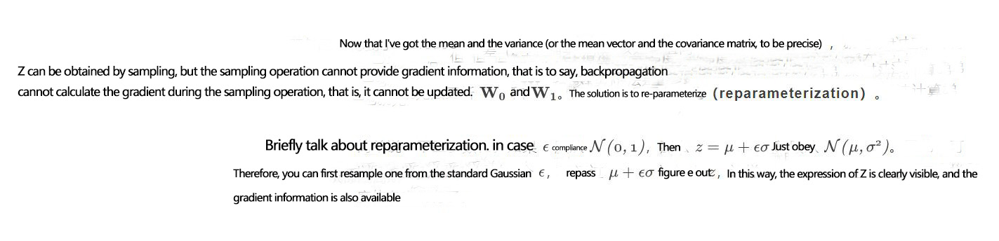
The decoder of VGAE is also a simple inner-product, no different from the decoder of GAE.

1.3.3 How to learn

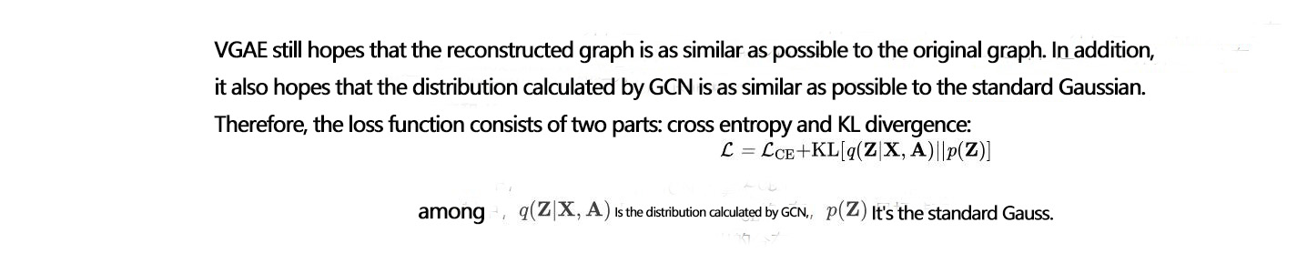
However, the optimization goal in the paper is this:

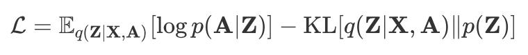
This is the optimization goal written in the lower bound of the variation. The first term is the expectation, and the second term is the KL divergence.

1.4 Effect analysis

Kipf and Welling conducted effect analysis on three data sets, and the task was link prediction. For details, see the following table:

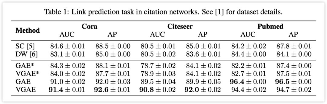
It can be seen that the effect of the (variational) graph autoencoder on the three data sets is very good. However, pay attention to the GAE* and VGAE* with asterisks. These two models do not have input features, that is, nodes. The features are one-hot vectors. In this case, the effect of the (variational) graph autoencoder is not only not better than SC and DW, but even has a point difference.

However, Kipf and Welling pointed out in the paper that SC and DW do not support input features, so being able to use input features is one of the features of VGAE.

The above is an introduction to the pioneering paper Variational Graph Auto-Encoders. Next, let’s look at some applications of graph auto-encoders in the past two years.

Paper Title: Graph Convolution Matrix Completion

Paper source: KDD 2018

Link to the paper:

https://www.kdd.org/kdd2018/files/deep-learning-day/DLDay18_paper_32.pdf

2.1 Overview of the paper

This is an article by Kipf that solves the matrix completion problem in the recommendation system as the second work, published in KDD in 18 years.

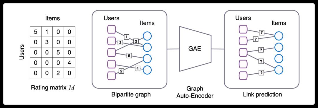
This article proposes that the matrix completion task can be regarded as a link prediction problem on the graph, that is, users and items form a bipartite graph, and the edges on the graph represent the interaction between the corresponding user and the item, so the matrix completion problem changes It became a problem of predicting the edges on this bipartite graph.

In order to solve the link prediction problem on the users-items bipartite graph, this article proposes a graph autoencoder framework GCMC based on message passing on the bipartite graph, and introduces side information and analyzes the side information for the recommendation system The impact of cold start.

2.2 Detailed model

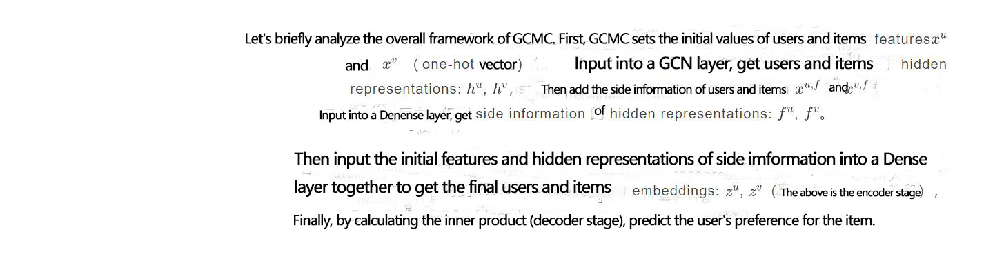
The detailed calculation method for each step is given below.

First, the calculation method of the GCN layer is as follows:

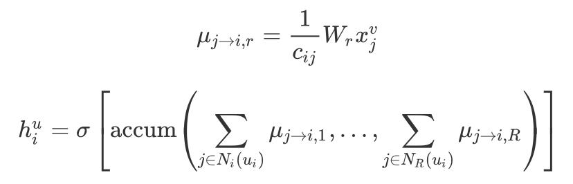
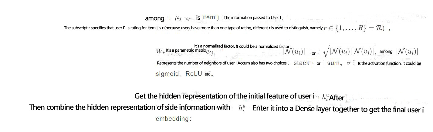
Among them, the right type represents the Dense layer where the hidden representation of the side information is obtained, and the left type represents the Dense layer where the final embedding is obtained.

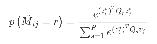
After getting the embeddings of users and items, use the following formula to predict the probability that user i's score on item j belongs to r:

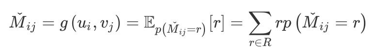
Finally, GCMC's prediction of user i's rating of item j is:

2.3 Effect analysis

The author uses 6 data sets, which can be divided into 3 categories:

The comparison method only uses the features of users or items: ml-100k

Neither GCMC nor comparison methods use side information: ml-1m, ml-10m

The side information of Users and items is presented in the form of graph: Flixster, Douban, YahooMusic

Experimental results:

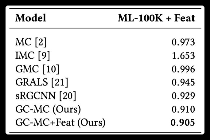
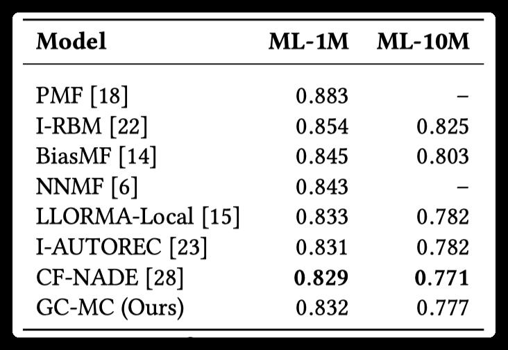
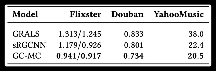
The experimental results show that when there is side information, the effect of GCMC is better than other methods, especially when the side information exists in the form of graph, the effect of GCMC is more obvious. When there is no side information, GCMC also showed competitive results.

The author also analyzed the impact of side information on cold start. In the article, ml-100k is used as an example to artificially reduce the number of ratings for some users, and then compare the effects of GCMC with and without side information.

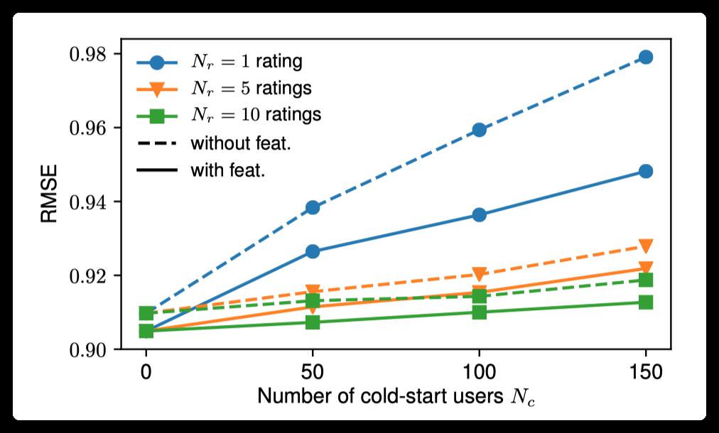
As can be seen from the above figure, GCMC using side information is more effective, and as the number of cold start users increases, the effect of introducing side information is more obvious.

2.4 Summary

This paper treats the matrix completion task in the recommendation system as a link prediction task on the graph, and uses the graph autoencoder to introduce side information. It surpasses some SOTA methods on some benchmark data sets, and also analyzes the side Information for the help of cold start.

cGraphCAR